Optimization and Simulated Annealing

While working on the puzzle game Dollar Shuffle, I had the thought that all programmers have from time to time: “Why don’t I make the computer do this for me?” Specifically I was thinking about the individual puzzles. I had already created around 30 by hand but it was quickly becoming tedious. Why not set up a script to generate levels automatically?

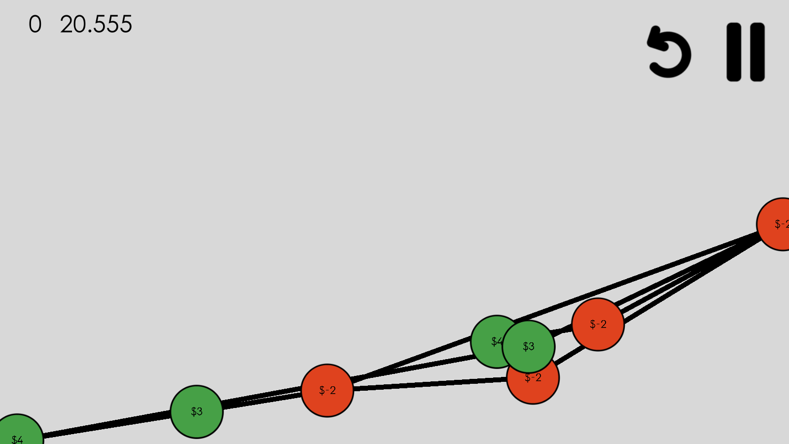
Creating the graph was the easy part. With judicious use of randi and randf I created a collection of nodes, connected them randomly, and distributed points amongst them. There was one problem with this: the graphs were ugly.

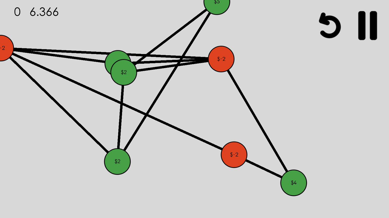
Horrifically, terribly ugly. Confusing, too.

This is how I began delving into the world of graph drawing and the aesthetics of it. What does it mean for a graph to look “good”? How can one create an algorithm to fulfill that definition?

Graph Drawing

The Wikipedia page for Graph Drawing lists a few “quality measures” of a graph but only a few of those applied to this situation:

• The crossing number, or the number of pairs of edges that cross over one another
• The angular resolution, or the sharpness of the smallest angle between two lines
• Deviation in edge length
• Deviation in distance between nodes
• Nodes too close to border of screen

With these well defined measures, we can create a cost function: a mathematical formula used to “grade” a current setup. This function is used to optimize the graph. To maximize the good-looking-ness of the graph, we minimize the output of this function. Below is an example cost function only implementing the last 3 measures listed above:

# Total cost of graph -- This could have been one int, but separating them
# make debugging easier
var costs = [0, 0, 0]

# For each node in the graph...
for node in graph.keys():
    
    # Get location of current node
    var node_loc = graph[node]["loc"]
    
    # NODE DISTRIBUTION 
    # For each pair of nodes in graph...
    var other_nodes = graph.keys()
    other_nodes.erase(node)
    for pair in other_nodes:
        
        # Add the square inverse of nodes' distance
        # Small distance means high cost
        costs[0] += L1 / max(node_loc.distance_squared_to(graph[pair]["loc"]), 0.0001)
    
    # BORDER DISTANCE
    # Calculate distance squared to top, bottom, left, and right edges
    var t = max(node_loc.distance_squared_to(Vector2(node_loc.y, BORDER_T)), 0.0001)
    var b = max(node_loc.distance_squared_to(Vector2(node_loc.y, BORDER_B)), 0.0001)
    var l = max(node_loc.distance_squared_to(Vector2(node_loc.x, BORDER_L)), 0.0001)
    var r = max(node_loc.distance_squared_to(Vector2(node_loc.x, BORDER_R)), 0.0001)
    # Add inverses of these vars to total, scaled by l2
    # Small distances mean high cost
    costs[1] += L2 * (1.0 / t + 1.0 / b + 1.0 / l + 1.0 / r)
    
    # For each connection that node has...
    for conn in graph[node]["conns"]:
        # EDGE LENGTHS
        # Add the square distance between the connected nodes
        # Large distances mean high cost
        var edge_len = node_loc.distance_squared_to(graph[conn]["loc"])
        costs[2] += L3 * edge_len

return costs[0] + costs[1] + costs[2]

The biggest stumbling block for optimization problems in general is local minima and maxima. These are points that represent a best setup for a small range of possible setups, but not the best overall. For instance, if our optimization problem was finding the lowest point in a curve, a local minimum would be the bottom of a small valley that still sits above a lower valley. For our situation, these are layouts that seem like the best solution, but even better ones exist if we could make some adjustments that might make the graph worse in the interim. Not getting stuck in local minima is key to getting an optimized graph, so let’s explore one optimization technique that avoids them.

Simulated Annealing

Simulated annealing is a process where a setup – the layout of the graph’s nodes in our case – is randomly tweaked and compared to the previous setup using the cost function. If it’s better, we keep the new setup. Otherwise, we select which one to keep randomly, with the probability of keeping the old one proportional to how much better it is. This small element of randomness helps to avoid local minima. Repeat this a few thousand times and, eventually, a significantly better setup is found. It’s a process not unlike natural selection: a change is made and, if it’s better, it outlives its predecessor. By performing simulated annealing on our graph we can produce a layout that minimizes the quality measures listed above.

# Define a starting "temperature", which limits how far nodes can move 
var temp = 0.85

# Start by randomly distributing all nodes
for node in graph.keys():
    graph[node]["loc"] = Vector2(randf(), randf())

# For the predefined number of trials...
for index in range(TRIALS):

    var graph_new = generate_candidate(graph, temp)
    # Calculate the probability of new layout replacing old one.  If new layout
    # has lower cost, replacement is guaranteed
    var cost_new = cost(graph_new)
    var prob = exp((cost_current - cost_new) * PROB_CONST / temp)
    if randf() < prob:
        graph = graph_new
        cost_current = cost_new

The key part of this algorithm is hidden in the phrase “randomly tweaked”. At first, these random changes can be large. For instance, it could move a node a few hundred pixels in any direction. As the algorithm progresses the changes become more constrained. By the end of the algorithm it might be moving nodes 10 or 15 pixels. The reason for this – and the reason simulated annealing is an effective optimization technique – is that it allows the setup to break out of local minima and maxima early on in the process.

# For the predefined number of trials...
for index in range(TRIALS):

    # Same process as above...

# Reduce temperature at a predefined rate
temp *= D_TEMP

The final part of the puzzle (so to speak) is when to stop the annealing. A set number might lead to suboptimal graphs, or it could lead to wasting processor time on an already good graph. A better heuristic is keeping track of how many times in a row it doesn’t find a better layout. If this number gets too big, then the graph we have must be pretty good, so we can just break out. While this may mean not getting perfect graphs, that’s alright. As long as the produced layouts aren’t bad or confusing, that’s enough. We wouldn’t want players to wait for several minutes while the game generates each level!

# Start by randomly distributing all nodes
for node in graph.keys():
    graph[node]["loc"] = Vector2(randf(), randf())

# Define a starting "temperature", which limits how far nodes can move 
var temp = 0.85

# Create a counter for how often sequential layouts are rejected
var rejects = 0

var cost_current = cost(graph)

# While temp is above stopping threshold...
while temp > LIM_TEMP:
    
    # For the predefined number of trials...
    for index in range(TRIALS):
        
        var graph_new = generate_candidate(graph, temp)
        # Calculate the probability of new layout replacing old one.  If new layout
        # has lower cost, replacement is guaranteed
        var cost_new = cost(graph_new)
        var prob = exp((cost_current - cost_new) * PROB_CONST / temp)
        if randf() < prob:
            graph = graph_new
            cost_current = cost_new
            rejects = 0
        
        # Otherwise, increment the rejection counter
        else:
            rejects += 1
        
            # If rejection counter is too high, break out of this loop
            if rejects >= LIM_REJECT:
                rejects = 0
                break
    
    # Reduce temperature at a predefined rate
    temp *= D_TEMP

After the annealing process I also added a “fine tuning” step that added one additional quality measure. In this phase the cost function also considered how close any given node was to the edges. This was to make sure that the graphs being produced didn’t have nodes sitting on top of edges they weren’t connected to. This would have been confusing at best, and game-breaking at worst.

# Once main processing is done, do fine tuning
# Re-calculate cost of graph, now with edge-distance cost
cost_current = cost(graph, true)
# Only allow small changes
temp = 0.04

for index in range(FINE_TUNING_LOOPS):
    var graph_new = generate_candidate(graph, temp)
    # Only replace graph if new cost is lower
    var cost_new = cost(graph_new, true)
    if cost_new < cost_current:
        graph = graph_new
        cost_current = cost_new

I’m certainly not the first one to apply simulated annealing to graph drawing. In fact, almost all of my code was adapted from a research paper by Davidson and Harel. It turns out, simulated annealing has been used to make nice looking graphs on computers almost as long as graphs have been displayed on computers. All that was left for me to do was adapt that code into GDScript, the Godot game engine’s proprietary language.

All of these bits are put together in the graph_annealing.gd file in the Dollar Shuffle repo. Because the game is open source you’re free to take this code and play with it yourself!

Conclusion

Most of the time, going overboard on algorithms and over-engineering solutions is a bad idea. Because this was a project I created entirely for my own enjoyment I knew I could play around with some more complicated code. Implementing simulated annealing was a good challenge and got me back into my computer science headspace. Don’t be afraid of topics that seem complex and over your head – working though it step-by-step will teach you much!